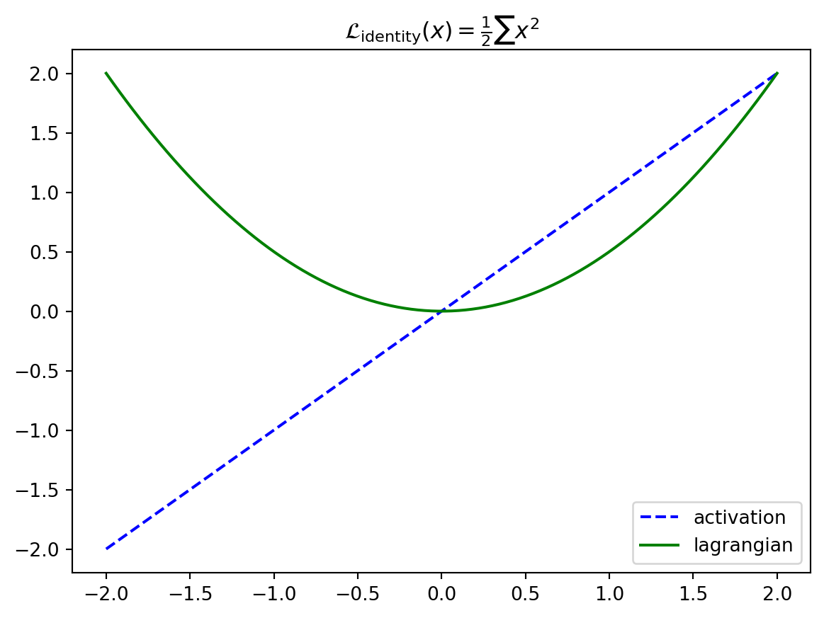
lagr_identity
lagr_identity (x:jax.Array)
The Lagrangian whose activation function is simply the identity.
| Type | Details | |
|---|---|---|
| x | Array | Input tensor |
| Returns | Float | Output scalar |
The well-behaved energy of associative memories is captured by the Lagrangian of the neurons
The dynamic state of each 🌀neuron layer is constrained by a convex Lagrangian.
Lagrangian functions are fundamental to the energy of 🌀neuron layers. These convex functions can be seen as the integral of common activation functions (e.g., relus and softmaxes). All Lagrangians are functions of the form:
\[\mathcal{L}(\mathbf{x};\ldots) \mapsto \mathbb{R}\]
where \(\mathbf{x} \in \mathbb{R}^{D_1 \times \ldots \times D_n}\) can be a tensor of arbitrary shape and \(\mathcal{L}\) can be optionally parameterized (e.g., the LayerNorm’s learnable bias and scale). Lagrangians must be convex and differentiable.
We want to rely on JAX’s autograd to automatically differentiate our Lagrangians into activation functions. For certain Lagrangians, the naively autodiff-ed function of the defined Lagrangian is numerically unstable (e.g., lagr_sigmoid(x) and lagr_tanh(x)). In these cases, we follow JAX’s documentation guidelines to define custom_jvps to fix this behavior.
Let’s look at what some of these Lagrangians look like in practice.
Though we define Lagrangians for an entire tensor, these special “elementwise Lagrangians” take a special form: they are simply the sum of the convex, differentiable function applied elementwise to the underlying tensor. This makes it easy to plot and visualize them.
lagr_identity (x:jax.Array)
The Lagrangian whose activation function is simply the identity.
| Type | Details | |
|---|---|---|
| x | Array | Input tensor |
| Returns | Float | Output scalar |
\[ \begin{align*} \mathcal{L}_\text{identity}(\mathbf{x}) &= \frac{1}{2} \sum_i x_i^2 \\ \partial_{x_i} \mathcal{L}_\text{identity}(\mathbf{x}) &= x_i \end{align*} \]
lagr_repu (x:jax.Array, n:float)
Rectified Power Unit of degree n
| Type | Details | |
|---|---|---|
| x | Array | Input tensor |
| n | float | Degree of the polynomial in the power unit |
| Returns | Float | Output scalar |
\[ \begin{align*} \mathcal{L}_\text{RePU}(\mathbf{x}; n) &= \frac{1}{n} \sum_i \max(x_i, 0)^n \\ \partial_{x_i} \mathcal{L}_\text{RePU}(\mathbf{x}; n) &= \max(x_i, 0)^{n-1} \end{align*} \]
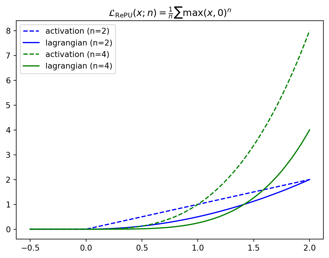
lagr_relu (x:jax.Array)
Rectified Linear Unit. Same as lagr_repu of degree 2
| Type | Details | |
|---|---|---|
| x | Array | Input tensor |
| Returns | Float | Output scalar |
\[ \begin{align*} \mathcal{L}_\text{relu}(\mathbf{x}) &= \frac{1}{2} \sum_i \max(x_i, 0)^2 \\ \partial_{x_i} \mathcal{L}_\text{relu}(\mathbf{x}) &= \max(x_i, 0) \end{align*} \]
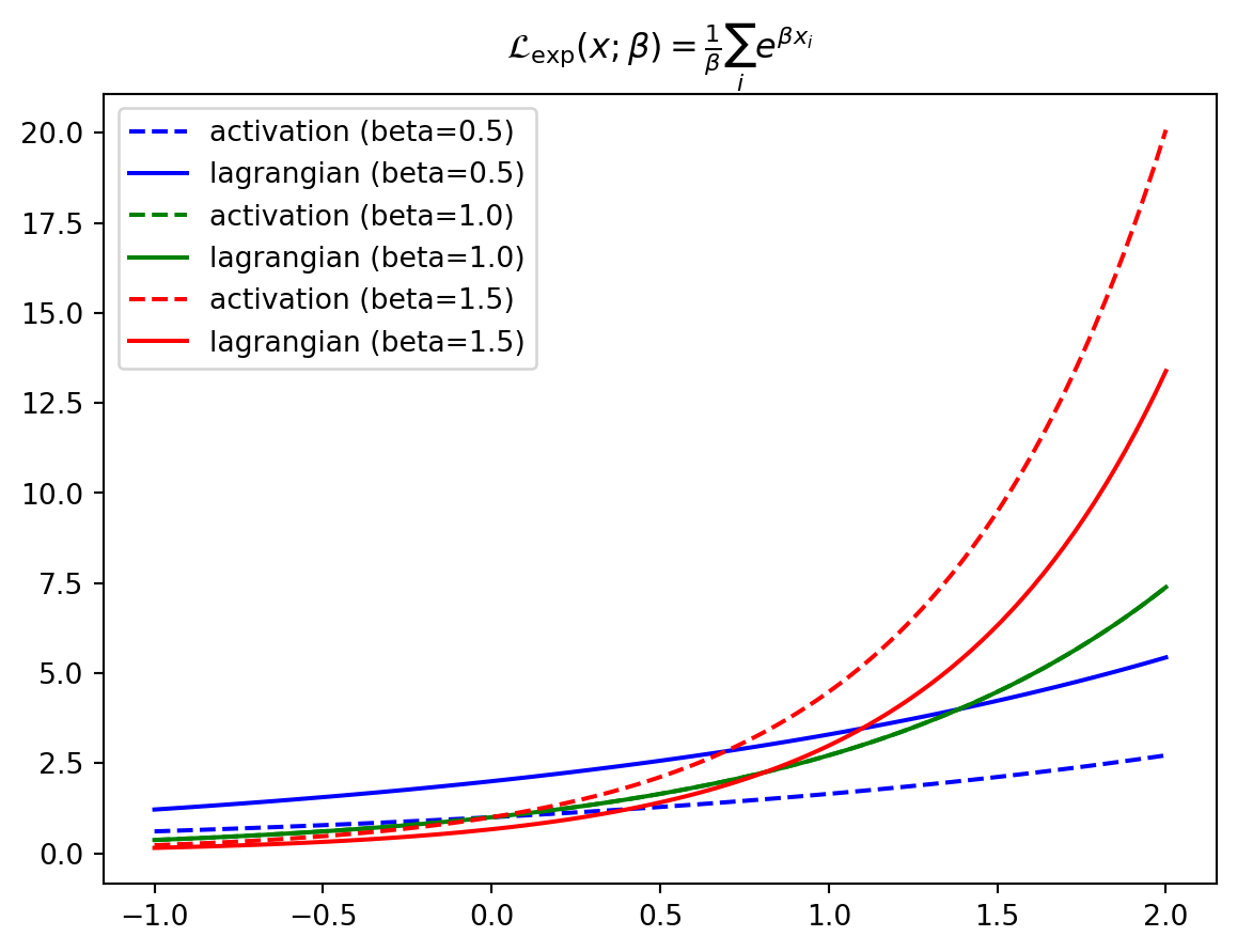
lagr_exp (x:jax.Array, beta:float=1.0)
Exponential activation function, as in Demicirgil et al.. Operates elementwise
| Type | Default | Details | |
|---|---|---|---|
| x | Array | Input tensor | |
| beta | float | 1.0 | Inverse temperature |
| Returns | Float | Output scalar |
\[ \begin{align*} \mathcal{L}_\text{exp}(\mathbf{x}; \beta) &= \frac{1}{\beta} \sum_i e^{\beta x_i} \\ \partial_{x_i} \mathcal{L}_\text{exp}(\mathbf{x}; \beta) &= e^{\beta x_i} \end{align*} \]
lagr_tanh (x:jax.Array, beta:float=1.0)
Lagrangian of the tanh activation function
| Type | Default | Details | |
|---|---|---|---|
| x | Array | Input tensor | |
| beta | float | 1.0 | Inverse temperature |
| Returns | Float | Output scalar |
\[ \begin{align*} \mathcal{L}_\text{tanh}(\mathbf{x}; \beta) &= \frac{1}{\beta} \sum_i \log(\cosh(\beta x_i)) \\ \partial_{x_i} \mathcal{L}_\text{tanh}(\mathbf{x}; \beta) &= \tanh(\beta x_i) \end{align*} \]
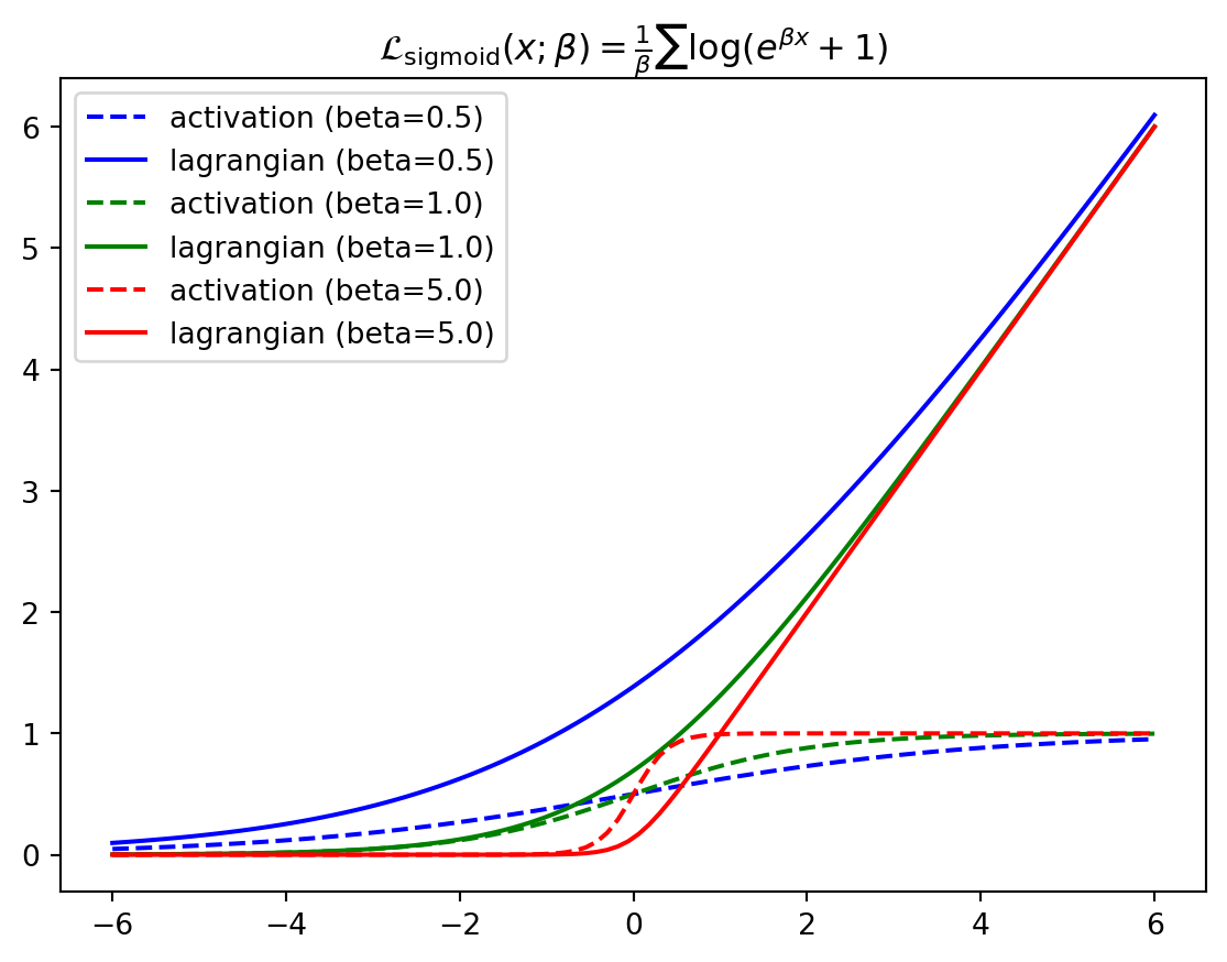
lagr_sigmoid (x:jax.Array, beta:float=1.0)
The lagrangian of the sigmoid activation function
| Type | Default | Details | |
|---|---|---|---|
| x | Array | Input tensor | |
| beta | float | 1.0 | Inverse temperature |
| Returns | Float | Output scalar |
\[ \begin{align*} \mathcal{L}_\text{sigmoid}(\mathbf{x}; \beta) &= \frac{1}{\beta} \sum_i \log(e^{\beta x_i} + 1) \\ \partial_{x_i} \mathcal{L}_\text{sigmoid}(\mathbf{x}; \beta) &= \frac{1}{1+e^{-\beta x_i}} \end{align*} \]
However, we can also have Lagrangians defined on neuron layers where every unit competes. There are many forms of activation functions in modern Deep Learning with this structure; e.g., softmaxes, layernorms, etc. normalize their input by some value. These activation functions can similarly be described by Lagrangians (and there is a nice interpretation of these kinds of activation functions as competing hidden units, but it is harder to plot them.
lagr_softmax (x:jax.Array, beta:float=1.0, axis:int=-1)
The lagrangian of the softmax – the logsumexp
| Type | Default | Details | |
|---|---|---|---|
| x | Array | Input tensor | |
| beta | float | 1.0 | Inverse temperature |
| axis | int | -1 | Dimension over which to apply logsumexp |
| Returns | Float | Output scalar |
\[ \begin{align*} \mathcal{L}_\text{softmax}(\mathbf{x}; \beta) &= \frac{1}{\beta} \log \sum_i e^{\beta x_i} \\ \partial_{x_i} \mathcal{L}_\text{softmax}(\mathbf{x}; \beta) &= \frac{e^{\beta x_i}}{\sum_j e^{\beta x_j}} \end{align*} \]
We plot its activations (the softmax) for a vector of length 10 below.

 lagr_layernorm (x:jax.Array, gamma:float=1.0,
                 delta:Union[float,jax.Array]=0.0, axis:int=-1,
                 eps:float=1e-05)
*Lagrangian of the layer norm activation function.
gamma must be a float, not a vector.*
| Type | Default | Details | |
|---|---|---|---|
| x | Array | Input tensor | |
| gamma | float | 1.0 | Scale the stdev |
| delta | Union | 0.0 | Shift the mean |
| axis | int | -1 | Which axis to normalize |
| eps | float | 1e-05 | Prevent division by 0 |
| Returns | Float | Output scalar |
\[ \begin{align*} \mathcal{L}_\text{layernorm}(\mathbf{x}; \gamma, \delta) &= D \gamma \sqrt{\text{Var}(\mathbf{x}) + \epsilon} + \sum_i \delta_i x_i \\ \partial_{x_i} \mathcal{L}_\text{layernorm}(\mathbf{x}; \gamma, \delta) &= \gamma \frac{x_i - \text{Mean}(\mathbf{x})}{\sqrt{\text{Var}(\mathbf{x}) + \epsilon}} + \delta_i \end{align*} \]
 lagr_spherical_norm (x:jax.Array, gamma:float=1.0,
                      delta:Union[float,jax.Array]=0.0, axis:int=-1,
                      eps:float=1e-05)
Lagrangian of the spherical norm (L2 norm) activation function
| Type | Default | Details | |
|---|---|---|---|
| x | Array | input tensor | |
| gamma | float | 1.0 | Scale the stdev |
| delta | Union | 0.0 | Shift the mean |
| axis | int | -1 | Which axis to normalize |
| eps | float | 1e-05 | Prevent division by 0 |
| Returns | Float | Output scalar |
\[ \begin{align*} \mathcal{L}_\text{L2norm}(\mathbf{x}; \gamma, \delta) &= \gamma \sqrt{\sum_i x_i^2 + \epsilon} + \sum_i \delta_i x_i \\ \partial_{x_i} \mathcal{L}_\text{L2norm}(\mathbf{x}; \gamma, \delta) &= \gamma \frac{x_i}{\sqrt{\sum_j x_j^2 + \epsilon}} + \delta_i \end{align*} \]